This is an old revision of the document!
PAIREF in CCP4 - lunchtime byte
5 Jan 2023
In this short tutorial, we submit a paired refinement job using the PAIREF program, now distributed in the CCP4 suite. You can use our example data from interferon gamma from Paralichthys olivaceus (POLI) 1), PDB entry 6F1E.
Download example data
Download the archive with the example data and extract it in a folder - we will refer this folder as working folder. The archive contains:
- Structure model previously refined against data at 2.3 Å - poli67_webinar_2-3A.pdb.
- Merged diffraction data up to 1.9 Å - poli67_1-9A.mtz
- Unmerged diffraction data up to 1.9 Å - poli67_XDS_ASCII_1-9A.HKL
Open console in working directory
In Windows, find the CCP4 console in the Start menu and open it (see the screenshots below). In GNU/Linux or macOS, just open the terminal, assuming all the executables for CCP4 are available there.
Then go to the folder where your structure model and diffraction data are saved using the command cd. For example, if you saved those three files in folder C:/Users/Lab/PAIREF_tutorial_poli, write cd C:/Users/Lab/PAIREF_tutorial_poli into the console and press Enter.
Run PAIREF in command line
We will add three high-resolution shells step by step: 2.3-2.10 Å, 2.1-2.0 Å and 2.0-1.9 Å. Run PAIREF:
ccp4-python -m pairef --XYZIN poli67_webinar_2-3A.pdb --HKLIN poli67_1-9A.mtz -u poli67_XDS_ASCII_1-9A.HKL -r 2.1,2.0,1.9 -w 0.06 -p poli_webinar
Note: The structure model was refined using X-ray weight 0.06, we have to keep this setting to gain unbiased results.
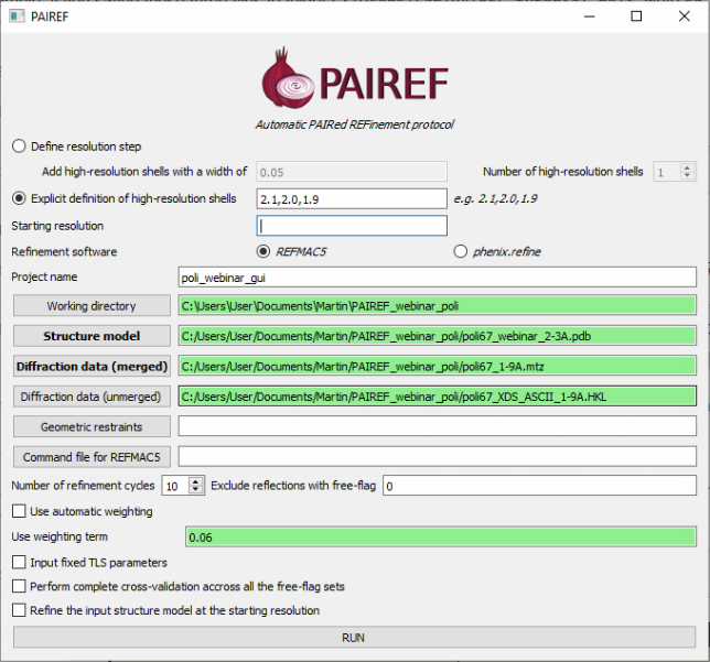
Run PAIREF using its graphical user interface
PAIREF provides a standalone graphical user interface (GUI) for intuitive setting of arguments without making up a command. For launching the PAIREF GUI, execute the following command:
ccp4-python -m pairef --gui
Interpretation of results
Follow the note ------> RESULTS AND THE CURRENT STATUS OF CALCULATIONS ARE LISTED IN A HTML LOG FILE in the program output and open the stated file in your preferred web browser (e.g. Firefox). The results should look similar to ours: https://pairef.fjfi.cvut.cz/docs/pairef_poli_webinar/PAIREF_poli_webinar.html.
The first thing that should be checked is whether the refinements have converged. Scroll at the very bottom of page, here you can see plots of Rwork and Rfree vs. refinement cycle. We can conclude that all the refinements have converged.
Rfree decreased after the addition of shells 2.3-2.10 Å and 2.1-2.0 Å:
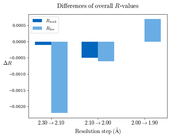
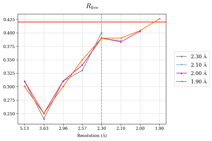
Since a perfect model gives an R-value of 0.42 against random data (i.e. pure noise) – assuming non-tNCS (translational non-crystallographic symmetry) data from a non-twinned crystal 2) – a higher R-value in the (current) high-resolution shell indicates either the involvement of high-resolution data without information content (the data are even worse than noise), or poor quality of the model, or the presence of tNCS. This is indicated for the shell 2.0-1.9 Å.
CC* a model-independent measure of noise is in the diffraction data. CC* is higher than CCwork in whole resolution range (except the shell 2.0-1.9 Å where CC* is undefined due to negative CC1/2. Thus, the overfitting was not indicated. To access overfitting, it is not needed to test set, so the comparison of CC* with CCwork is much better then with CCfree as CCwork is calculated on more data.
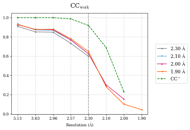
We can conclude that the high-resolution cutoff can be set to 2.0 Å.
Merging statistics:
#shell d_max  d_min   #obs  #uniq   mult.  %comp       <I>  <I/sI>    r_mrg   r_meas    r_pim   cc1/2   cc_ano     cc*
01     47.05   5.13  22367   1948   11.48  99.44     494.1    38.8    0.042    0.044    0.013   0.999  -0.214   0.9997
02      5.13   3.63  42232   3343   12.63  99.79     203.3    31.7    0.064    0.067    0.019   0.999  -0.163   0.9997
03      3.63   2.97  57138   4246   13.46  99.95      56.9    14.3    0.151    0.157    0.042   0.997  -0.166   0.9992
04      2.97   2.57  65007   5014   12.97  99.70      11.3     4.0    0.622    0.648    0.178   0.951  -0.025   0.9874
05      2.57   2.30  73887   5623   13.14  99.89       3.7     1.3    1.839    1.914    0.523   0.730  -0.014   0.9187
06      2.30   2.10  83129   6181   13.45  99.92       1.2     0.4    5.812    6.041    1.633   0.311   0.001   0.6888
07      2.10   2.00  49772   4021   12.38  98.51       0.3     0.1   16.989   17.721    4.963   0.027   0.008   0.2293
08      2.00   1.90  35920   4046    8.88  81.18       0.1     0.0   41.435   43.993   14.417  -0.132  -0.016   N/A
Contact
In case of any questions or problems, please do not hesitate and write us: m.maly #AT# soton.ac.uk.
Further reading
- More information about PAIREF settings and possibilities are explained in the documentation.
- Linking crystallographic model and data quality. P.A. Karplus & K. Diederichs (2012) Science 336:1030–3
- Assessing and maximizing data quality in macromolecular crystallography. P.A. Karplus & K. Diederichs (2015) Cur. Op. in Str. Biology 34:60–68
- Better models by discarding data? P.A. Karplus & K. Diederichs (2013) Acta Cryst. D59:1215–1222