Download presentation in PDF

In this short tutorial, we submit a paired refinement job using the PAIREF program, now distributed in the CCP4 suite. You can use our example data from interferon gamma from Paralichthys olivaceus (POLI) ¹⁾, PDB entry 6F1E.

Download the archive with the POLI data and extract it in a folder - we will refer this folder as working folder. The archive contains:

• Structure model previously refined against data at 2.3 Å - poli67_webinar_2-3A.pdb.
• Merged diffraction data up to 1.9 Å - poli67_1-9A.mtz
• Unmerged diffraction data up to 1.9 Å - poli67_XDS_ASCII_1-9A.HKL

The structure of POLI was originally refined at 2.3 Å resolution. Nevertheless, we will inspect an impact of the reflection beyond this high-resolution cutoff on the model quality, We have data processed up to 1.9 Å resolution. Thus, we will add three high-resolution shells step by step: 2.3-2.1 Å, 2.1-2.0 Å and 2.0-1.9 Å.

PAIREF is available within the CCP4I2 from the CCP4 version 8.0.013. Open CCP4I2 and go to Task Menu → Refinement → PAIREF to create a new PAIREF job.

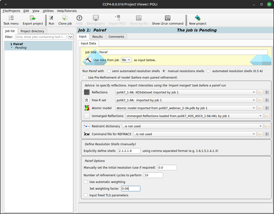
In the PAIREF window, we need to specify:

• How we want to add high-resolution shells - select “Run PAIREF with manual resolution shells” and put 2.1,2.0,1.9 to “Explicitly define shells…”
• Input merged diffraction data - import Reflections from poli67_1-9A.mtz and select intensities (I), not anomalous
• Free R set - import from poli67_1-9A.mtz
• Input structure model - import poli67_webinar_2-3A.pdb
• Input unmerged data - import poli67_XDS_ASCII_1-9A.HKL
• Uncheck “Use automatic weighting” and set weighting factor to 0.06 - from prior knowledge just for this particular data set

Your window should look like similarly to the screenshot below:

And now we can press Run and open the log file.

The results should look similar to ours: https://pairef.fjfi.cvut.cz/docs/pairef_poli_ccp4sw2023/PAIREF_poli_ccp4sw2023.html.

PAIREF ran all the calculation and did also an automatic suggestion of an optimal high-resolution cut off. Let's check the table on top of the HTML log file:

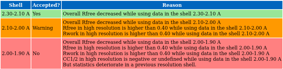
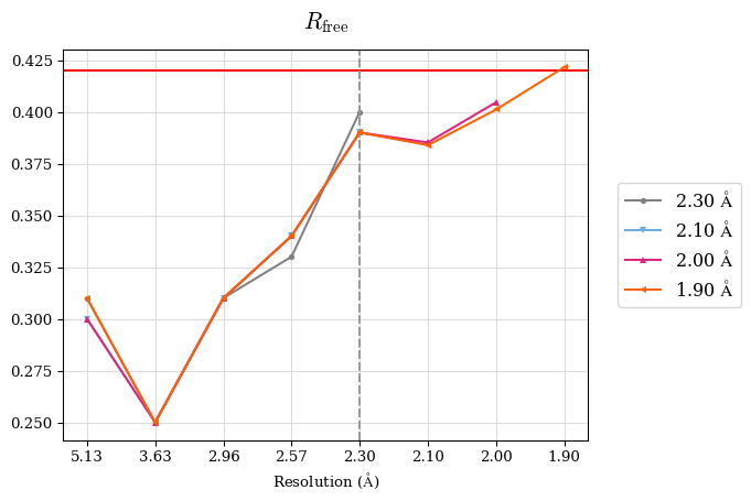
The suggestion is based on the results plotted in the following graphs. Overall Rfree decreased for all the three high-resolution shells that denotes model improvement:

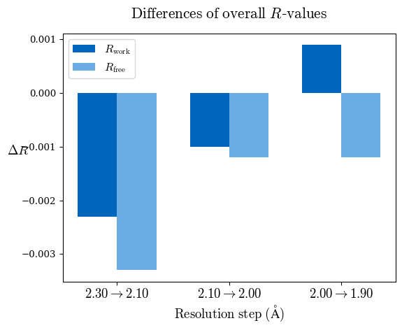
However, we should take into account multiple criteria. Since a perfect model gives an R-value of 0.42 against random data (i.e. pure noise) – assuming non-tNCS (translational non-crystallographic symmetry) data from a non-twinned crystal ²⁾ – a higher R-value in the (current) high-resolution shell indicates either the involvement of high-resolution data without information content (the data are even worse than noise), or poor quality of the model, or the presence of tNCS. This is indicated for the shell 2.0-1.9 Å.

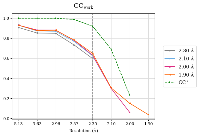
CC* is a model-independent measure of noise is in the diffraction data. For this data set, CC* is higher than CCwork in the whole resolution range, except the shell 2.0-1.9 Å where CC* is undefined due to negative CC1/2. That means overfitting was not indicated but the shell 2.0-1.9 Å should be discarded because these data are very noisy. Note that to access overfitting, it is not needed to use test set, so the comparison of CC* with CCwork is much better than with CCfree as CCwork is calculated on more data.

We should also check whether the refinements have converged. Scroll at the very bottom of page, here you can see plots of Rwork and Rfree vs. refinement cycle. We can conclude that all the refinements have converged, indeed.

We can conclude that the high-resolution limit of the data is ca. 2.1 Å.

Merging statistics:

#shell d_max  d_min   #obs  #uniq   mult.  %comp       <I>  <I/sI>    r_mrg   r_meas    r_pim   cc1/2   cc_ano     cc* 
01     47.05   5.13  22367   1948   11.48  99.44     494.1    38.8    0.042    0.044    0.013   0.999  -0.214   0.9997
02      5.13   3.63  42232   3343   12.63  99.79     203.3    31.7    0.064    0.067    0.019   0.999  -0.163   0.9997
03      3.63   2.97  57138   4246   13.46  99.95      56.9    14.3    0.151    0.157    0.042   0.997  -0.166   0.9992
04      2.97   2.57  65007   5014   12.97  99.70      11.3     4.0    0.622    0.648    0.178   0.951  -0.025   0.9874
05      2.57   2.30  73887   5623   13.14  99.89       3.7     1.3    1.839    1.914    0.523   0.730  -0.014   0.9187
06      2.30   2.10  83129   6181   13.45  99.92       1.2     0.4    5.812    6.041    1.633   0.311   0.001   0.6888
07      2.10   2.00  49772   4021   12.38  98.51       0.3     0.1   16.989   17.721    4.963   0.027   0.008   0.2293
08      2.00   1.90  35920   4046    8.88  81.18       0.1     0.0   41.435   43.993   14.417  -0.132  -0.016   N/A

It is also possible to run PAIREF in the command line. The job described here could be executed using the following command:

ccp4-python -m pairef --XYZIN poli67_webinar_2-3A.pdb --HKLIN poli67_1-9A.mtz -u poli67_XDS_ASCII_1-9A.HKL -r 2.1,2.0,1.9 -w 0.06 -p poli

In case of any questions or problems, please do not hesitate and write us: m.maly #AT# soton.ac.uk.

• Paired refinement under the control of PAIREF. M. Maly, K. Diederichs, J. Dohnalek, P. Kolenko (2020) IUCrJ 7
• More information about PAIREF settings and possibilities are explained in the documentation.

• Linking crystallographic model and data quality. P.A. Karplus & K. Diederichs (2012) Science 336:1030–3
• Assessing and maximizing data quality in macromolecular crystallography. P.A. Karplus & K. Diederichs (2015) Cur. Op. in Str. Biology 34:60–68
• Better models by discarding data? P.A. Karplus & K. Diederichs (2013) Acta Cryst. D59:1215–1222